Introduction

Since the release of Microsoft Excel® 2007 there has been a logical object called a Table. This object has a default name and its rows and columns can automatically grow and shrink to reflect the data. Tables have an optional summary row, shown at the bottom of the table, that can show statistics like Sum, Average and Count. Sharperlight uses the Table object as a container for the query data that comes from a Table Formula.

Table Formulas use an anchor formula in the worksheet to reference the related Excel Table, the query template name and the filter cell references. This formula can be moved anywhere on the worksheet and it will continue to function provide the Excel Table name and query template exist.

The formatting of a Table Formula data set in Excel is purely controlled by the formatting options in Excel. The formatting controls in the Query Builder only affect web content published to the Web Channel.

Practices

Let’s take a look at the Table Formula.

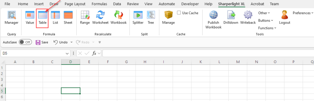
Select a cell to make it the anchor cell, and click the Table icon on the SharperLight ribbon.

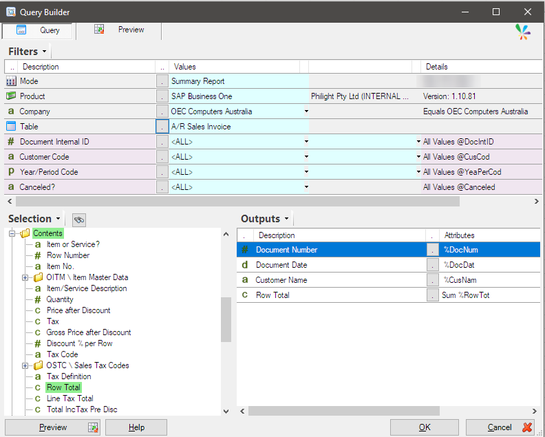
Build a query like this:

The extracted dataset is displayed as a table.

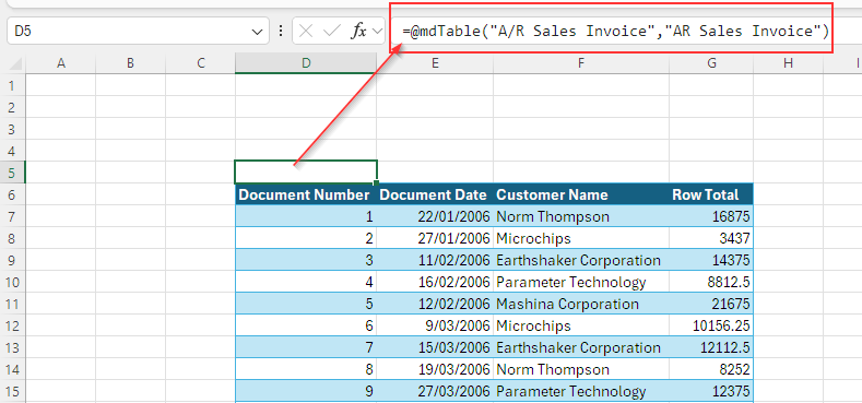
The query definition can be opened for editing by double-clicking the cell where the Table Formula is defined.

Then, the Cell Reference can be used to specify values for filters and drive the query execution.

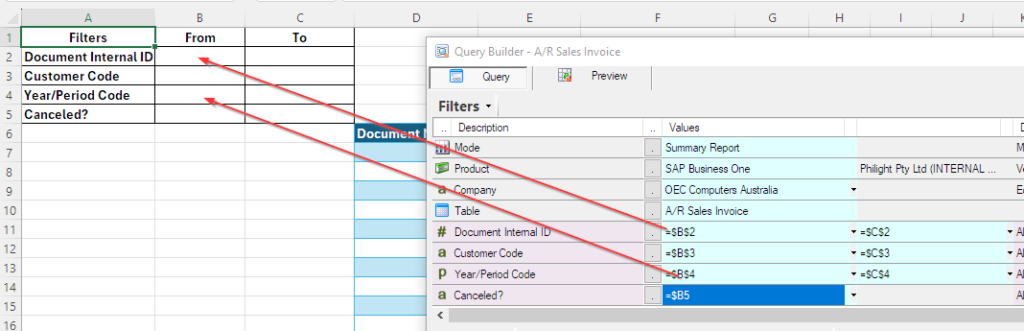
The Table Formula is updated with the cell reference details.

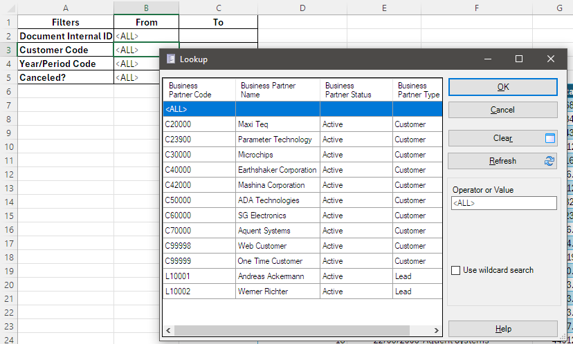
Once the cell reference is set up, you can open the lookup dialog by double-clicking the reference cell.

Afterword

This is one of the SharperLight Excel Add-in formulas, and we hope it will be helpful for your business.

See also the post for Value Formula.

See also the post for more information.